Introducing pyflowtool
When I was in my junior year of university, I took ESCI100A (Introduction to Environmental Sciences) with Professor Matthias Hain. This class focused very much on quantitative and systems approaches to understanding the environment and I found it fascinating.
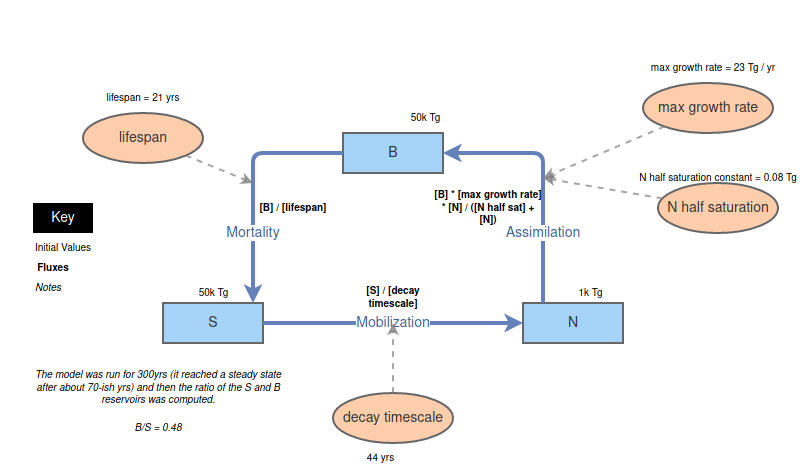
What interested me most about the class was the use of the InsightMaker tool. InsightMaker is oriented towards modeling physical systems by making use of "inventories" and "flows." The former represent variables -- water in a tank, CO2 in the atmosphere, or some other (typically conserved) physical quantity. The latter represent formulae for describing the change in an inventory. Flows can connect from one inventory to another, transferring between the two, or may be connected only on one end. I've attached a picture of an example model below.
This tool is really fun to use since you can very quickly make complex models of real environmental processes and, in a classroom environment, it can really help understand what is happening. I did, however, find that the web interface and the cumbersome method of inputting formulae detracted from the experience. While these downsides did not typically get in the way, they were major hindrances if you were on a deadline or in a rush.
Another concern I had with InsightMaker was that it did not permit the use of volumes of data (like a 3D grid). While outside the scope of the tool, I felt that it would be a welcome improvement to an already elegant piece of software.
These problems (and enhancements) led me to become interested in developing my own version -- one which would run natively on my own machine and which could be more optimized for performance. Additionally, I wanted to be able to use gridded variables in order to prototype more complex models without writing boilerplate code. Furthermore, I wanted to try my hand at implementing different numeric integrator schema from the book Numeric Recipes in C.
I did not attempt any of this until a month or so after completing the course when I became curious about Python's decorator syntax. This feature seemed to me to be the perfect approach to implementing a python version of InsightMaker. Put simply, decorators are functions which take functions as parameters and return functions as outputs. I felt that they would be useful because they would be able to define flows in a convenient and pythonic way.
I started out with the following idea for how I wanted things to work: the user defines inventories using strings, and then defines functions to act as flows. These flow functions should take in an argument for time and another argument representing the model’s state. The result of these design choices can be seen below:
declare_inventory('A')

# ...

@declare_flow('Flow Name')
def some_flow(t: float, m: dict) -> float:
    # ...
    return 0

# ...

run_model()
From the above plan, I think it is obvious why I thought decorators were a good idea -- they made the resulting model code more elegant.
At this point, I was confident that I could make a working implementation, albeit without a graphical interface. The pyflowtool library ended up only taking around nine hours over the course of a couple of days to write, and I think that the result is fairly good (although it still needs some work for reasons that will explain in a moment).
This tool works by creating an internal dictionary which tracks all of the flows, inventories, and other objects that are needed to make a model. There are seven functions which pyflowtool exposes as its API:
pf_reset_model()This resets the library's state.pf_make_display(name:str, invs=[], fs=[], vs=[], label=None)This declares a plot and accepts a list of inventories and flows to plot (with time as the horizontal axis).pf_run_model(start=0, stop=10, step=1)Calling this runs the model from a start time to a stop time.pf_make_inventory(name, value=0.0, nickname=None)This allows the user to declare inventories with a name, an optional value, and a nickname (used for plotting).pf_flow(name=None, source=None, sink=None, clamp=True)This is the decorator used to declare a flow and takes an optional name, source, and sink. Additonally, the user can optionally specify if they want the flow to be clamped to positive values.pf_var(name=None)This is a decorator which declares a variable.pf_setup(_func)This is a decorator which is used bypf_run_modelto initialze everything before running the model.
These are all (with the exception of pf_var) straightforward to use but I'll still do a walkthough of an example just to preempt some future questions. A script which uses pyflowtool will start with the usual:
from pyflowtool import *
We are going to try to replicate the model shown at the start of the article, so we will actually begin by defining come constants:
max_growth_rate = 0.2; n_half_sat = 1000.0; lifespan = 10
decay_timescale = 30; denitr_frac = 0.05; leaching_frac = 0.05
regrowth_time = 50
Now, we can define our setup function. Note how we never explicitly run the setup function. One of the quirks of python is that defining a function technically executes code (unlike in compiled languages like C and so defining init_model with the pf_setup decorator causes the pf_setup decorator to be executed, thereby registering the init_model function with the pyflowtool library.
@pf_setup
def init_model():
	# define inventories
	pf_make_inventory('B', value=30000)
	pf_make_inventory(['S', 'N'], value=[90000, 1000])
	# make displays
	pf_make_display('Inventories', invs=['B', 'S', 'N'], label='Inventories (TgN)')
The above snippet begins by defining init_model and calling the decorator pf_setup on it. Inside the init_model function, we declare two inventories using two different conventions to showcase the flexibility of the pf_make_inventory function. We then make a display which will be called "Inventories" and will plot the B, S, and N inventories. The label parameter is used to specify the label of the vertical axis.
Now, we can begin by defining our first flow: Assimilation.
@pf_flow(name='Assimilation', source='N', sink='B')
def assimilation(t, m):
	return max_growth_rate * m['B'] * ( 1 / ( n_half_sat + m['N'] ) ) * m['N']
This flow returns a float and accepts a float named t and a dictionary named m (although the types are not explicitly specified). Notice how the decorator pf_flow takes optional parameters for the name, sink, and source of the flow. If a sink is specified, the flow will subtract from that inventory, and if a source is specified then the flow will add to that inventory. Neither of these parameters is required.
We continue on with defining eight additional flows (which, for brevity's sake, I will not show here).
Finally, we can run the model like so:
Is, Fs, Vs = pf_run_model(start=1700, stop=2000, step=0.1)
The pf_run_model function executes the model and returns the values of all flows, variables, and inventories at each timestep. It will also produce all displays (usually as matplotlib pop-up windows) before exiting.
Let’s take a moment to discuss variables. These are quantities computed each timestep from flows and inventories and can be used as outputs or diagnostics. They are a prominent feature of the actual InsightMaker tool. They do, however, represent a problem: since variables depend on flows and inventories, and since flows and inventories depend on variables, calculating them at each timestep is challenging. I suspect that the best solution is to simply always compute variables at the start of the timestep.
There are also some numerical issues -- the version of the code discussed at this point simply uses Euler's method for integration, and therefore may exhibit numeric instability. I still need to improve this.
This project has sat on my github untouched for more than a year now, and I feel that it is time to complete it. My goals for this project (before I set it aside again) are to:
- Fix the problem with variables.
- Improve the timestepping.
- Add support for gridded variables.
- Add support for various interpolation schemes for variables.
- Add support for intra-volume flows.
- Maybe add GPU compute support.
As I accomplish these steps I’ll post updates here.